實作 MNIST 手寫數字即時多重辨識— — 使用 OpenCV 與 TensorFlow Lite(可在電腦與樹莓派運行)並用 AutoKeras 超輕鬆建立 CNN 模型
機器學習與深度學習近年一直非常熱門,不過總歸來說,只要掌握合適的資料集和套件,要建立模型是相對容易的。真正的問題在於:你要怎麼拿它們投入實用呢?特別是當你的模型一次只能辨認一張圖時,你要如何從一個畫面中辨識出多重圖像?你要如何讓模型在裝置上實際運行,發揮出它們從一開始就該扮演的角色?
MNIST 手寫數字資料集出現於 1998 年,含有六萬張訓練圖像及一萬張測試圖像,每張都是 28 x 28 灰階圖片。由於處理起來相對容易,如今被當成視覺辨識的入門經典範例,只要用一般的 CNN 模型就能得到相當好的預測效果,而且模型不會很大。若我們將它轉成 TensorFlow Lite 格式,那麼不管在電腦或樹莓派上都能十分順暢地執行。

此外,基於手寫數字的特性,只要辨識畫面中只有數字跟空白背景,要分離背景跟數字就不難。這使得我們不太需要改變原本的資料集跟模型,只要做些影像預處理即可。
當然,基於 MNIST 資料集的特質,你可能得讓攝影機拍攝照明充足的紙張,並用簽字筆寫下長寬相當的數字。太瘦長或歪斜的筆跡會比較難得到正確結果。
本文討論的內容包括:
- 用 AutoKeras 建立一個 Keras CNN 模型
- 將模型轉換為 TensorFlow Lite 版
- 理解 TensorFlow Lite 模型如何呼叫
- 用 OpenCV 預處理畫面,找出可能的數字位置
- 對可能的數字做預測並顯示結果
如果你只想知道怎麼執行這個範例,直接看下一節即可。當中的原理我會從後面繼續。
快速上手
到這個 repo 下載兩個檔案:
- mnist.tflite
- mnist_tflite_live_detection.py
把它們放在同一個資料夾內。
然後在電腦或樹莓派上安裝 NumPy 與 OpenCV :
pip3 install --upgrade numpy opencv-python在 Windows 執行請於結尾加上 --user。在 Linux 則在前面加 sudo。
然後是 TensorFlow Lite Runtime 的 wheel 檔,到下面這裡下載符合你平台與系統的版本:
例如我的 Win10 電腦使用 Python 3.9,就用 tflite_runtime-2.5.0.post1-cp39-cp39-win_amd64.whl(cp39 代表 Python 3.9,amd64 即 x64);樹莓派 OS Buster 用 xxx-cp37-cp37m-linux_armv7l.whl(樹莓派 2~4B 為 ARMv8 架構),樹莓派 OS Bullseye 則用 xxx-cp39-cp39-linux_armv7l.whl,以此類推:
pip3 install 路徑/tflite_runtime-2.5.0.post1-cp37-cp37m-linux_armv7l.whl使用 Raspberry Pi Imager 安裝樹莓派 OS 時,預設會安裝最新的 Buster,這是針對樹莓派 4B 設計的。若使用舊型板子或想要維持相容性,請在 Imager 選擇 Raspberry Pi OS Legacy。
最後你只要接上 webcam,執行 mnist_tflite_live_detection.py 即可:
使用 AutoKeras 建立 CNN 模型
我知道,你可以用單純的 Keras 建立類似的模型,但用 AutoKeras 做起來非常省事,而且效果比我用一模一樣結構的 Keras 模型更好(AutoKeras 會在選擇模型以後,合併訓練集/驗證集再跑一次訓練,並在合適的訓練週期停止)。

我使用 AutoKeras 1.0.16 post1,它搭配的是 Tensorflow 2.5.2:
pip3 install --upgrade autokeras==1.0.16post1安裝 AutoKeras 會一併安裝 Numpy、scikit-learn、TensorFlow 在內的套件。有趣的是在電腦上安裝時,TensorFlow 2.5 要求的 Numpy 版本不得超過 1.19.5,但後來試過用最新的也行(我現在用 1.22.0)。
TensorFlow 2.x 必須安裝在 Python 3.6 64-bit 以上環境。
寫這篇不久後 AutoKeras 推出 1.0.17,支援到 TF 2.8.0,但訓練行為上有些改變。我覺得 1.0.16 的表現略好一點,所以個人還是建議找個環境裝這種版本。
mnist_tflite_trainer.py 的內容即為模型產生器:
TF_LITE_MODEL = './mnist.tflite'  # 要產生的 TF Lite 檔名
SAVE_KERAS_MODEL = True  # 是否儲存 Keras 原始模型import autokeras as ak
import tensorflow as tf
from tensorflow.keras.datasets import mnist# 載入 MNIST dataset
(x_train, y_train), (x_test, y_test) = mnist.load_data()# 訓練 AutoKeras 模型
clf = ak.ImageClassifier(max_trials=1, overwrite=True)
clf.fit(x_train, y_train)# 用測試集評估模型
loss, accuracy = clf.evaluate(x_test, y_test)
print(f'\nPrediction loss: {loss:.3f}, accurcy: {accuracy*100:.3f}%\n')# 匯出 Keras 模型
model = clf.export_model()
model.summary()# 儲存 Keras 模型
if SAVE_KERAS_MODEL:
    model.save('./mnist_model')# 將模型轉為 TF Lite 格式
converter = tf.lite.TFLiteConverter.from_keras_model(model)# 你也可以讀取已儲存的 Keras 模型來轉換:
# converter = tf.lite.TFLiteConverter.from_saved_model('./mnist_model')
tflite_model = converter.convert()# 儲存 TF Lite 模型
with open(TF_LITE_MODEL, 'wb') as f:
    f.write(tflite_model)
可以看到用 AutoKeras 非常單純,基本上只要幾行程式就能建模。當然這裡運用了一點內行知識:ak.ImageClassifier() 會從三個預設模型開始試驗,第一個是標準 CNN 模型,對 MNIST 圖像來說就非常夠用了。因此我們將 max_trials 參數設為 1,表示只需試驗第一個模型即可。
就個人經驗,ak.ImageClassifier() 第二個預設模型 ResNet50 對 MNIST 效果不如 CNN,而第三個 EfficientNet B7 已經到了殺雞用牛刀的程度,訓練起來也非常耗時。所以實際上也就沒必要去嘗試這些模型了。
程式輸出結果如下:
Trial 1 Complete [00h 04m 14s]
val_loss: 0.03911824896931648

Best val_loss So Far: 0.03911824896931648
Total elapsed time: 00h 04m 14s
Epoch 1/21
1875/1875 [==============================] - 8s 4ms/step - loss: 0.1584 - accuracy: 0.9513
Epoch 2/21
1875/1875 [==============================] - 8s 4ms/step - loss: 0.0735 - accuracy: 0.9778
Epoch 3/21
1875/1875 [==============================] - 8s 4ms/step - loss: 0.0616 - accuracy: 0.9809
Epoch 4/21
1875/1875 [==============================] - 8s 4ms/step - loss: 0.0503 - accuracy: 0.9837
Epoch 5/21
1875/1875 [==============================] - 8s 4ms/step - loss: 0.0441 - accuracy: 0.9860
Epoch 6/21
1875/1875 [==============================] - 8s 4ms/step - loss: 0.0414 - accuracy: 0.9864
Epoch 7/21
1875/1875 [==============================] - 8s 4ms/step - loss: 0.0383 - accuracy: 0.9872
Epoch 8/21
1875/1875 [==============================] - 8s 4ms/step - loss: 0.0331 - accuracy: 0.9893
Epoch 9/21
1875/1875 [==============================] - 8s 4ms/step - loss: 0.0325 - accuracy: 0.9893
Epoch 10/21
1875/1875 [==============================] - 8s 4ms/step - loss: 0.0307 - accuracy: 0.9901
Epoch 11/21
1875/1875 [==============================] - 8s 4ms/step - loss: 0.0305 - accuracy: 0.9899
Epoch 12/21
1875/1875 [==============================] - 8s 4ms/step - loss: 0.0287 - accuracy: 0.9906
Epoch 13/21
1875/1875 [==============================] - 8s 4ms/step - loss: 0.0258 - accuracy: 0.9917
Epoch 14/21
1875/1875 [==============================] - 8s 4ms/step - loss: 0.0243 - accuracy: 0.9920
Epoch 15/21
1875/1875 [==============================] - 8s 4ms/step - loss: 0.0254 - accuracy: 0.9915
Epoch 16/21
1875/1875 [==============================] - 9s 5ms/step - loss: 0.0243 - accuracy: 0.9920
Epoch 17/21
1875/1875 [==============================] - 8s 4ms/step - loss: 0.0231 - accuracy: 0.9922
Epoch 18/21
1875/1875 [==============================] - 8s 4ms/step - loss: 0.0218 - accuracy: 0.9924
Epoch 19/21
1875/1875 [==============================] - 8s 4ms/step - loss: 0.0213 - accuracy: 0.9932
Epoch 20/21
1875/1875 [==============================] - 9s 5ms/step - loss: 0.0226 - accuracy: 0.9927
Epoch 21/21
1875/1875 [==============================] - 8s 4ms/step - loss: 0.0197 - accuracy: 0.9938

313/313 [==============================] - 1s 3ms/step - loss: 0.0387 - accuracy: 0.9897

Prediction loss: 0.039, accuracy: 98.970%

Model: "model"
_________________________________________________________________
Layer (type)                 Output Shape              Param #
=================================================================
input_1 (InputLayer)         [(None, 28, 28)]          0
_________________________________________________________________
cast_to_float32 (CastToFloat (None, 28, 28)            0
_________________________________________________________________
expand_last_dim (ExpandLastD (None, 28, 28, 1)         0
_________________________________________________________________
normalization (Normalization (None, 28, 28, 1)         3
_________________________________________________________________
conv2d (Conv2D)              (None, 26, 26, 32)        320
_________________________________________________________________
conv2d_1 (Conv2D)            (None, 24, 24, 64)        18496
_________________________________________________________________
max_pooling2d (MaxPooling2D) (None, 12, 12, 64)        0
_________________________________________________________________
dropout (Dropout)            (None, 12, 12, 64)        0
_________________________________________________________________
flatten (Flatten)            (None, 9216)              0
_________________________________________________________________
dropout_1 (Dropout)          (None, 9216)              0
_________________________________________________________________
dense (Dense)                (None, 10)                92170
_________________________________________________________________
classification_head_1 (Softm (None, 10)                0
=================================================================
Total params: 110,989
Trainable params: 110,986
Non-trainable params: 3
我在電腦上使用 GPU 訓練,所以兩次訓練加起來只要略少於 7 分鐘,不過在一般電腦上用 CPU 也很難超過一小時。可發現模型對訓練集跟測試集的預測表現相當,準確率都逼近 99%,損失值(MSE)也低於 0.04。
這模型是個由 2D 卷積層、全域 2D 池化層、扁平層、dropout 以及全連接層構成,匯出為 Keras 模型後為 611 KB,轉換為 TF Lite 後縮減為 432 KB。
TensorFlow Lite 的差別在哪?
將 Keras 模型轉換為 TF Lite 時,它會做以下三件事:
- 訓練後量化(quantization):將權重與啟動函數的資料從 32 位元浮點數轉為 16 位元浮點數、16 位元整數或 8 位元整數,好減少模型大小並加快運算速度。
- 修剪非必要權重(pruning):移除模型中對預測結果影響很小的權重。
- 權重分群(clustering):將每一層的權重分類成 N 個叢集,以該叢集的中心值(centroid value)當成權重。這等於是能壓縮模型的大小。
換言之,TF Lite 模型藉由稍微犧牲模型的表現來換取更短的推論(做預測的)時間與更小的體積。
檢視 TF Lite 模型的表現

既然模型預測能力在壓縮後可能會打點折扣,我們可以載入 TF Lite 模型,檢視此模型對 MNIST 測試集的表現,順便了解一下如何操作它。
現在我們要使用 mnist_tflite_model_test.py(它會用到 TensorFlow、scikit-learn 以及 matplotlib):
TF_LITE_MODEL = './mnist.tflite'  # 模型名稱import tensorflow as tf
from tensorflow.keras.datasets import mnist
from pprint import pprint# 只載入 MNIST 測試集
(_, _), (x_test, y_test) = mnist.load_data()
print('test image shape:', x_test.shape)
print('test label shape:', y_test.shape)
print('')# 載入 TF Lite 模型並檢視輸出入節點
print('Loading', TF_LITE_MODEL, '...\n')
interpreter = tf.lite.Interpreter(model_path=TF_LITE_MODEL)
interpreter.allocate_tensors()
input_details = interpreter.get_input_details()
output_details = interpreter.get_output_details()# 印出輸出入張量的細節
print('input details:')
pprint(input_details)
print('')
print('output details:')
pprint(output_details)
print('')# 為了對測試集資料做預測,修改輸出入節點的資料形狀
interpreter.resize_tensor_input(input_details[0]['index'], x_test.shape)
interpreter.resize_tensor_input(output_details[0]['index'], y_test.shape)
interpreter.allocate_tensors()
input_details = interpreter.get_input_details()
output_details = interpreter.get_output_details()print('new input shape:', input_details[0]['shape'])
print('new output shape:', output_details[0]['shape'])
print('')# 進行推論
print('Predicting...')
interpreter.set_tensor(input_details[0]['index'], x_test)
interpreter.invoke()
predicted = interpreter.get_tensor(output_details[0]['index']).argmax(axis=1)# 檢視預測指標
from sklearn.metrics import accuracy_score, mean_squared_error
print('Prediction accuracy:', accuracy_score(y_test, predicted).round(4))
print('Prediction MSE:', mean_squared_error(y_test, predicted).round(4))
print('')# 和真實分類比較並產生報告
from sklearn.metrics import classification_report
print(classification_report(y_test, predicted))# 畫出測試集前 40 張圖以及其預測結果
import matplotlib.pyplot as plt
fig = plt.figure(figsize=(6, 3))
for i in range(40):
    ax = fig.add_subplot(4, 10, i + 1)
    ax.set_axis_off()
    ax.set_title(f'{predicted[i]}')
    plt.imshow(x_test[i], cmap='gray')
plt.tight_layout()
plt.savefig('./mnist-model-test.jpg')
plt.show()
TF Lite 會以解釋器(interpreter)的形式包裝在模型之上:

為了最佳化 TF Lite 模型表現,你得分配適當的記憶體給它的張量(tensor),也就是輸出入的資料結構:
interpreter.allocate_tensors()接著你可以檢視模型的輸出入張量:
input_details = interpreter.get_input_details()
output_details = interpreter.get_output_details()
下面是程式用 pprint 模組印出 input_details 和 output_details 的內容:
input details:
[{'dtype': <class 'numpy.uint8'>,
  'index': 0,
  'name': 'input_1',
  'quantization': (0.0, 0),
  'quantization_parameters': {'quantized_dimension': 0,
                              'scales': array([], dtype=float32),
                              'zero_points': array([],dtype=int32)},
  'shape': array([ 1, 28, 28]),
  'shape_signature': array([-1, 28, 28]),
  'sparsity_parameters': {}}]output details:
[{'dtype': <class 'numpy.float32'>,
  'index': 16,
  'name': 'Identity',
  'quantization': (0.0, 0),
  'quantization_parameters': {'quantized_dimension': 0,
                              'scales': array([], dtype=float32),
                              'zero_points': array([],dtype=int32)},
  'shape': array([ 1, 10]),
  'shape_signature': array([-1, 10]),
  'sparsity_parameters': {}}]
可以看到 input_details 和 output_details 其實會告訴你模型的輸出入資訊:
- 輸入 (1, 28, 28) (uint8) 資料,也就是一個陣列裡的一張圖,模型會將之轉換為 int32
- 輸出 (1, 10) (float32) 資料,即對 10 個分類的預測概率(probability),模型會從 int32 將它轉換出來
這樣的資料形狀每次可以接收一筆資料,並做出一次預測。但現在我們已經知道測試集有多大,所以我們可以修改輸出入節點的形狀:
interpreter.resize_tensor_input(input_details[0]['index'], x_test.shape)
interpreter.resize_tensor_input(output_details[0]['index'], y_test.shape)
重新對張量分配記憶體後,可看到輸出入形狀變成如下:
new input shape: [10000    28    28]
new output shape: [10000    10]
這麼一來就不必用迴圈輪流推論每一張圖的數字了。後面我們就必須這麼做,因為在實際對影像做預測時,我們不會知道究竟有多少數字需要預測。
接著我們便可將測試集資料傳入輸入張量,並要模型進行推論:
# 寫入資料
interpreter.set_tensor(input_details[0]['index'], x_test)# 推論
interpreter.invoke()# 讀取預測結果
predicted = interpreter.get_tensor(output_details[0]['index']).argmax(axis=1)
程式會產生所有預測標籤 — — 既然預測概率陣列的索引剛好等於預測數字本身,我們直接呼叫 argmax(axis=1) 取出陣列中最大概率的索引即可。在這之後,程式會將預測結果和測試集實際標籤做比較:
Predicting...
Prediction accuracy: 0.9897
Prediction MSE: 0.1737              precision    recall  f1-score   support           0       0.99      1.00      0.99       980
           1       0.99      1.00      0.99      1135
           2       0.99      0.98      0.99      1032
           3       0.99      0.99      0.99      1010
           4       0.98      0.99      0.99       982
           5       0.99      0.99      0.99       892
           6       0.99      0.99      0.99       958
           7       0.98      0.99      0.99      1028
           8       0.99      0.99      0.99       974
           9       1.00      0.98      0.99      1009    accuracy                           0.99     10000
   macro avg       0.99      0.99      0.99     10000
weighted avg       0.99      0.99      0.99     10000
可見預測的 MSE 損失值變高了,但準確率仍然接近 99%,在所有分類都是如此。
此程式也會產生並儲存一張圖片,顯示測試集前 40 個數字與它們的預測結果,這就是本文一開始你看到的那張圖。
以靜態影像展示 OpenCV 的預處理
mnist_tflite_detection.py 會讀取一張靜態影像,做必要的預處理後交由 TF Lite 模型進行推論。它也會在過程中儲存一系列的影像,讓我們能更清楚觀察各步驟。
本篇我們不會特別解釋 OpenCV API,這本身就和任何 Python 套件一樣,是足以寫一本書的題材。以下只要先注意,OpenCV 的彩色影像是 BGR 格式,而且座標是高度在前、寬度在後。
我們的測試影像如下:
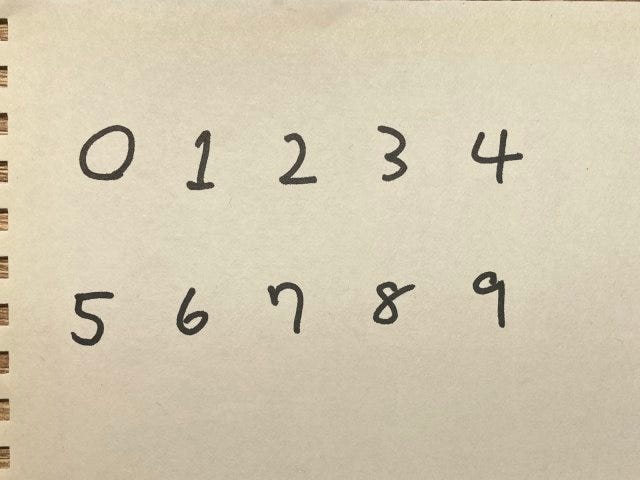
TEST_FILE = './test.jpg'  # 要測試的影像檔名
TF_LITE_MODEL = './mnist.tflite'  # TF Lite 模型
IMG_BORDER = 40  # 要忽略辨識的影像邊緣寬度
DETECT_THRESHOLD = 0.7  # 顯示預測結果的門檻 (70%)
LABEL_SIZE = 0.7  # 顯示預測值的字體比例 (70%)
RUNTIME_ONLY = True  # 使用 TF Lite Runtimeimport cv2
import numpy as np# 載入 TF Lite 模型
if RUNTIME_ONLY:
    from tflite_runtime.interpreter import Interpreter
    interpreter = Interpreter(model_path=TF_LITE_MODEL)
else:
    import tensorflow as tf
    interpreter = tf.lite.Interpreter(model_path=TF_LITE_MODEL)# 準備模型
interpreter.allocate_tensors()
input_details = interpreter.get_input_details()
output_details = interpreter.get_output_details()# 讀取輸入長寬
INPUT_H, INPUT_W = input_details[0]['shape'][1:3]# 要用於形態學閉運算的 kernel
MORPH_KERNEL = cv2.getStructuringElement(cv2.MORPH_RECT, (5, 5))# 讀取影像並取得長寬
img = cv2.imread(TEST_FILE, cv2.IMREAD_COLOR)
IMG_H, IMG_W = img.shape[:2]# 將影像轉為灰階
img_gray = cv2.cvtColor(img, cv2.COLOR_BGR2GRAY)
cv2.imwrite('./01-gray.jpg', img_gray)# 影像二值化 (轉為黑白)
_, img_binary = cv2.threshold(img_gray, 0, 255, cv2.THRESH_BINARY_INV | cv2.THRESH_OTSU)
cv2.imwrite('./02-binary.jpg', img_binary)# 做形態學閉運算去除黑雜訊
img_binary = cv2.morphologyEx(img_binary, cv2.MORPH_CLOSE, MORPH_KERNEL)
cv2.imwrite('./03-binary-morph.jpg', img_binary)# 圈出畫面中的輪廓
contours, _ = cv2.findContours(img_binary, cv2.RETR_EXTERNAL, cv2.CHAIN_APPROX_SIMPLE)# 拷貝影像 (以便展示結果)
img_binary_copy = img_binary.copy()
img_binary_result_copy = img_binary.copy()# 走訪所有輪廓
for contour in contours:
    x, y, w, h = cv2.boundingRect(contour)

    # 在輪廓上畫框
    cv2.rectangle(img_binary_copy, (x, y), (x + w, y + h), (255, 255, 255), 2)

    # 如果輪廓太靠近邊緣,忽略它
    if x < IMG_BORDER or x + w > (IMG_W - 1) - IMG_BORDER or y < IMG_BORDER or y + h > (IMG_H - 1) - IMG_BORDER:
        continue

    # 如果輪廓太大或太小,也忽略它
    if w < INPUT_W // 2 or h < INPUT_H // 2 or w > IMG_W // 2 or h > IMG_H // 2:
        continue

    # 擷取出輪廓內的影像
    img_digit = img_binary[y: y + h, x: x + w]

    # 在該影像周圍補些黑邊
    r = max(w, h)
    y_pad = ((w - h) // 2 if w > h else 0) + r // 5
    x_pad = ((h - w) // 2 if h > w else 0) + r // 5
    img_digit = cv2.copyMakeBorder(img_digit, top=y_pad, bottom=y_pad, left=x_pad, right=x_pad, borderType=cv2.BORDER_CONSTANT, value=(0, 0, 0))

    # 調整影像為模型輸入大小
    img_digit = cv2.resize(img_digit, (INPUT_W, INPUT_H), interpolation=cv2.INTER_AREA)    # 做預測
    interpreter.set_tensor(input_details[0]['index'], np.expand_dims(img_digit, axis=0))
    interpreter.invoke()
    predicted = interpreter.get_tensor(output_details[0]['index']).flatten()

    # 讀取預測標籤及其概率
    label = predicted.argmax(axis=0)
    prob = predicted[label]

    # 若概率低於門檻就忽略之
    if prob < DETECT_THRESHOLD:
        continue    # 印出預測結果、概率與數字的位置
    print(f'Detected digit: [{label}] at x={x}, y={y}, w={w}, h={h} ({prob*100:.3f}%)')

    # 在另一個影像拷貝的數字周圍畫框以及顯示標籤
    cv2.rectangle(img_binary_result_copy, (x, y), (x + w, y + h), (255, 255, 255), 1)
    cv2.putText(img_binary_result_copy, str(label), (x + w // 5, y - h // 5), cv2.FONT_HERSHEY_COMPLEX, LABEL_SIZE, (255, 255, 255), 1)# 顯示結果 (所有輪廓, 以及最後預測出來的數字)
cv2.imshow('Contours on binary image', img_binary_copy)
cv2.imwrite('./04-binary-contours.jpg', img_binary_copy)
cv2.imshow('MNIST detection result', img_binary_result_copy)
cv2.imwrite('./05-mnist-detection.jpg', img_binary_result_copy)# 在使用者按任何鍵後關閉視窗
cv2.waitKey(0)
cv2.destroyAllWindows()
程式開頭有一個 RUNTIME_ONLY 參數,設為 True 時會使用 TF Lite Runtime(這讓你能在樹莓派上執行而不必安裝 TensorFlow 2,特別是樹莓派 OS 仍然以 32-bit 為主流),設為 False 則會用標準 TensorFlow 內附的 TF Lite。
色彩的預處理
這支程式會在同目錄下產生一系列圖片。首先是用 cv2.cvtColor() 將原圖轉為灰階,將 RGB 三色通道減少為單色:

接著做二值化(thresholding),也就是將灰階像素 0~255 的值以某個分界點轉為非黑即白:
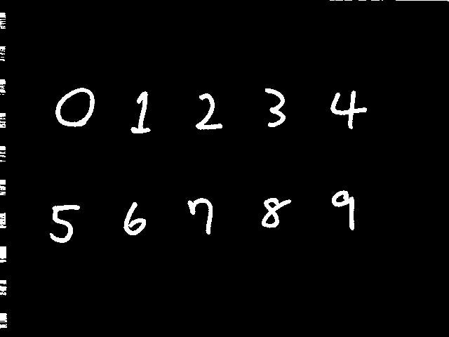
我們在呼叫 cv2.threshold() 函式時指定二值化的方式為 cv2.THRESH_BINARY_INV,也就是反轉黑白,這樣黑色的字跡會變成白色,符合 MNIST 資料集的圖檔。但同時我們還加上了 cv2.THRESH_OTSU 旗標,也就是套用大津二值化(Otsu’s method)來自動決定閥值(要轉為黑或白的分界點)。
一般而言大津二值化運作良好,但因光線或其他因素,你或許也會想自行手動設定。這時語法可改成如下:
cv2.threshold(img_gray, 160, 255, cv2.THRESH_BINARY_INV)這會將閥值設為 160,值比這低的像素轉為白色,較高的則轉為黑色。換言之,閥值越大使得被判定為白字的區域會越大。
接著我們呼叫 cv2.morphologyEx() 來做形態學閉運算(morphological closing):
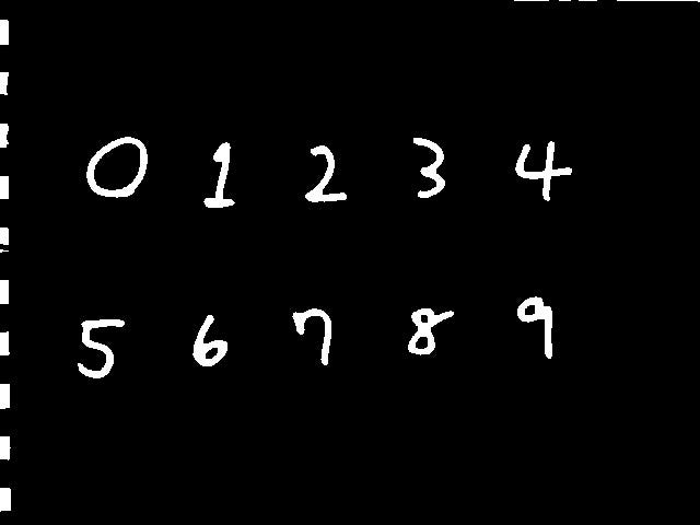
在此形態學閉運算會做兩件事:
- 膨脹(dilation):用前面提供的 5 x 5 kernel 均勻擴大白色區域。
- 腐蝕(erosion):用同一個 kernel 縮小白色區域的邊緣。
kernel 是 5 x 5 矩陣,裡面所有值都是 1,OpenCV 會用這個大小為單位來擴增和吃掉白色區域。簡單來說,這實際上的效果就是字跡中小於 5 x 5 的黑色雜點會在白色區域膨脹時被吃掉,然後再讓白字瘦身回到原本的程度,使字跡的邊緣會變得更平滑、字跡寬度稍微變粗。這樣對於後面的模型辨識應該會比較有利。
找出輪廓
若要在一個畫面中找出可能的數字,有個基本做法叫做移動窗格(sliding window):
- 決定一個大小的窗格,並讓它在畫面上移動、掃描不同區域。
- 將窗格內的區域輸入模型,看看是否能得到某個數字的高概率。
但這麼做有些問題:首先是你必須用不同大小的窗格重複掃描並做預測,這在效能上是個負擔,此外還得解決不同窗格「偵測到」同一個數字時的重複結果。
有些著名的影像辨識模型試著解決這個問題。YOLO(You Only Look Once)將整張畫面視為迴歸問題,計算每一個窗格可能包含目標的信心分數,而 SSD(Single Shot MultiBox Detector)則使用一個 CNN 來抽取特徵並畫出框。雖然做法稍有不同,兩者都會用非極大值抑制(non-maximum suppression)來消除重疊的框,保留最有可能的那個。
當然,這些模型使用的訓練影像也就得事先標註好目標物的位置,模型才有辦法學習如何從新畫面找出特定的東西。我們的模型訓練時只假設畫面是固定大小且只有一個數字,因此就必須用別的方法。
幸好,我們的情境比較單純,我們假設鏡頭前只有一張寫著數字的白紙,可以用 cv2.findContours() 把可能的數字輪廓圈起來:
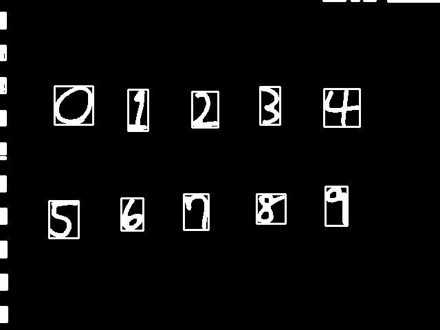
程式用 cv2.boundingRect() 將輪廓轉為 x, y, w, h 座標格式,然後在這些位置畫一個白色方框。可以看到除了數字以外,畫面邊緣也有一些地方(比如紙張的齒孔)被框起來了。目前我們的簡單解法是要程式忽略畫面邊緣 40 像素寬度的東西,以免紙張邊緣產生不正常的預測結果(畢竟模型沒有能力預測「非數字」)。
推論數字
程式會選擇忽略太大或太小的框,然後將框內的影像擷取出來。但這還有另一個問題:輪廓框會緊貼著數字,但 MNIST 的圖像在數字周圍有些「留黑」。若直接將輪廓內的數字拿來預測,效果就會沒那麼理想。
因此程式會做以下的額外處理:
- 在輪廓區域的短邊填入額外像素,使圖片的長寬相等。
- 在長寬額外加入 1/5 邊長的空白,讓數字置中。
- 將圖片縮到 28 x 28。
要注意的是模型的輸入形狀是 (1, 28, 28)(這回我們沒有修改它),而圖片本身是 (28, 28),所以你得替它增加一個維度:
np.expand_dims(img_digit, axis=0)這也可以寫成
np.array([img_digit])或tf.convert_to_tensor([img_digit]) # 必須用標準 TF
最後只要看數字的最大預測概率是哪一個數字、有沒有過門檻,把框和文字畫在畫面上就成了:
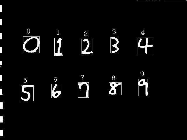
程式也會在 REPL 印出偵測到的數字以及其位置、概率:
Detected digit: [5] at x=71, y=292, w=43, h=54 (100.000%)
Detected digit: [6] at x=176, y=288, w=32, h=47 (100.000%)
Detected digit: [8] at x=373, y=282, w=42, h=43 (99.861%)
Detected digit: [7] at x=267, y=282, w=36, h=52 (99.974%)
Detected digit: [9] at x=473, y=271, w=32, h=57 (99.852%)
Detected digit: [2] at x=279, y=133, w=38, h=52 (99.997%)
Detected digit: [1] at x=186, y=130, w=29, h=60 (99.874%)
Detected digit: [4] at x=471, y=129, w=52, h=55 (100.000%)
Detected digit: [3] at x=378, y=126, w=29, h=55 (100.000%)
Detected digit: [0] at x=79, y=125, w=56, h=56 (100.000%)
其實要是數字的排列位置可以預期(比如一定寫在同一行)的話,還可以像 OCR 一樣把整個數字解讀出來。不過這邊就到此即可。
Webcam 即時辨識
mnist_tflite_live_detection.py 是前一個程式的即時版,運作原理其實一模一樣,只是輸入影像換成了自 webcam 取得的一格畫面而已,而且框和預測數字會顯示在原始的彩色影像上:
TF_LITE_MODEL = './mnist.tflite'  # TF Lite 模型
IMG_W = 640  # webcam 畫面寬度
IMG_H = 480  # webcam 畫面高度
IMG_BORDER = 40
DETECT_THRESHOLD = 0.7
CONTOUR_COLOR = (0, 255, 255)  # 輪廓框的顏色 (BGR)
LABEL_COLOR = (255, 255, 0)  # 文字標籤的顏色 (BGR)
LABEL_SIZE = 0.7
RUNTIME_ONLY = Trueimport cv2
import numpy as npif RUNTIME_ONLY:
    from tflite_runtime.interpreter import Interpreter
    interpreter = Interpreter(model_path=TF_LITE_MODEL)
else:
    import tensorflow as tf
    interpreter = tf.lite.Interpreter(model_path=TF_LITE_MODEL)interpreter.allocate_tensors()
input_details = interpreter.get_input_details()
output_details = interpreter.get_output_details()INPUT_H, INPUT_W = input_details[0]['shape'][1:3]MORPH_KERNEL = cv2.getStructuringElement(cv2.MORPH_RECT, (5, 5))# 開始擷取畫面
cap = cv2.VideoCapture(0)
cap.set(cv2.CAP_PROP_FRAME_WIDTH, IMG_W)
cap.set(cv2.CAP_PROP_FRAME_HEIGHT, IMG_H)while cap.isOpened():    # 取得一格畫面
    success, frame = cap.read()

    frame_gray = cv2.cvtColor(frame, cv2.COLOR_BGR2GRAY)

    _, frame_binary = cv2.threshold(frame_gray, 0, 255, cv2.THRESH_BINARY_INV | cv2.THRESH_OTSU)

    frame_binary = cv2.morphologyEx(frame_binary, cv2.MORPH_CLOSE, MORPH_KERNEL)

    contours, _ = cv2.findContours(frame_binary, cv2.RETR_EXTERNAL, cv2.CHAIN_APPROX_SIMPLE)

    for contour in contours:
        x, y, w, h = cv2.boundingRect(contour)

        if x < IMG_BORDER or x + w > (IMG_W - 1) - IMG_BORDER or y < IMG_BORDER or y + h > (IMG_H - 1) - IMG_BORDER:
            continue

        if w < INPUT_W // 2 or h < INPUT_H // 2 or w > IMG_W // 2 or h > IMG_H // 2:
            continue

        img = frame_binary[y: y + h, x: x + w]

        r = max(w, h)
        y_pad = ((w - h) // 2 if w > h else 0) + r // 5
        x_pad = ((h - w) // 2 if h > w else 0) + r // 5
        img = cv2.copyMakeBorder(img, top=y_pad, bottom=y_pad, left=x_pad, right=x_pad, borderType=cv2.BORDER_CONSTANT, value=(0, 0, 0))

        img = cv2.resize(img, (INPUT_W, INPUT_H), interpolation=cv2.INTER_AREA)        interpreter.set_tensor(input_details[0]['index'], np.expand_dims(img, axis=0))
        interpreter.invoke()
        predicted = interpreter.get_tensor(output_details[0]['index']).flatten()

        label = predicted.argmax(axis=0)
        prob = predicted[label]

        if prob < DETECT_THRESHOLD:
            continue

        cv2.rectangle(frame, (x, y), (x + w, y + h), CONTOUR_COLOR, 2)
        cv2.putText(frame, str(label), (x + w // 5, y - h // 5), cv2.FONT_HERSHEY_COMPLEX, LABEL_SIZE, LABEL_COLOR, 2)

    # 顯示處理過後的畫格
    cv2.imshow('MNIST Live Detection', frame)

    # 在使用者按 'q' 時結束
    if cv2.waitKey(1) == ord('q'):
        breakcap.release()
cv2.destroyAllWindows()
若你的裝置接有不只一台攝影機,可修改 cv2.VideoCapture(0) 的 0 為其他數字試試看。用筆電的前置攝影機也行。
我目前測試過在 Win10、樹莓派 3B+ 與 4B 都可以執行,而且由於模型簡單,640 x 480 在樹莓派 3B+ 也能維持流暢的禎數。以下是在樹莓派 3B+ 的執行畫面:

後記
對學習者而言,本範例的真正意義還是在於理解 OpenCV 和 ML/DL 模型能如何銜接起來,從多數入門教材的理論知識走向實用階段。其實實作 MNIST 手寫數字即時辨識不是新玩意,只是筆者在研究過程中一直找不到想要的範例,有許多還是在用正規 Keras 模型在跑。我試過這麼做也不是不可,只是若沒有開 GPU 支援,其推論延遲就會變得相當緩慢,所以這邊就沒介紹了。
TF Lite 模型並不支援 NVIDIA 顯卡加速,只能在 C++ 環境使用 Android 或 iOS 手機 GPU 來加速。此外如果跑複雜得多的 TF Lite 模型,例如 SSD-MobileNet 或 EfficientNet-Lite,在樹莓派上的表現也會明顯優於電腦。之後有機會的話,我們再來看如何透過 TF Lite 呼叫這些現成的物件偵測模型。
理論上樹莓派 2B 以及新的 Zero 2 W 也可以跑本篇的範例,它們都是 ARM8 架構。至於 Zero 一代,TF Lite Runtime 官方並沒有支援 ARM6 的版本,但有興趣的人或許可試試看有人自行產生的 wheel(2.3.1 版):
樹莓派 2 以後的版本其實都是 64 位元架構(aarch64),目前也有樹莓派 64-bit Beta OS,不過目前各種套件對這架構的支援並不普遍,所以可能還是得等等吧。
今天這邊就說到這啦!